Chapter 13 GLM Summary
13.1 Overview
Before we start going over todays lesson, let’s go over the general process of modelling.
- Model Selection (From Question)
- Model Fit
- Model Selection (By statistical reasoning, logic, and ecology)
- Model Validation/Diagnostics (some, or all of)
- Normaility of Errors
- Homogeneity of Variance
- Fixed X
- Indepence of Samples
- Correct Model Specification
- Model Visualization
13.2 Visualization
Visualizations specific to GLMs etc.
Before performing linear modeling…visualize!
With ecological questions, this exercise will help decide what type of modeling is required.
Here is what we mean, in Base R:
dotchart(mydata$length, groups = mydata$stage, ylab = "Stage", xlab = "Length")

scatterplot(mydata$length, mydata$width, groups = mydata$stage, by.groups = TRUE, smooth = FALSE, reg.line = FALSE, las = 1)

boxplot(length ~ stage, data = mydata, las = 1, ylab = "Length", xlab = "Stage")

pairs(mydata[3:5])
Note: Visualizations using ggplot2 are similar
13.3 GLM
General Linear Model
- Can be very simple (t.test, anova)
- Can be very complex (GLMM, ZIP, ZINB)
GLZ = Generalized Linear Model
- Now mostly referred to as GLM
The format of all modeling in R is very similar
lmb <- lm(y ~ x1, data = mydata) #simple linear regression
lmb <- glm(y ~ x1 + x2*x3, data = mydata) #GLM with 3 variables and an interaction term between variable 2 and 3
A typical GLM structure is formed as:
\[Y = \beta_{0} + \beta_{1}x_{1} + \beta_{2}x_{2} + \epsilon\] Where \(\epsilon\) is the predicted error, or, that varience in the data that can’t be explained by the factors \(x_{1}\), \(x_{2}\), etc.
We use the sample data residuals to estimate the predicted error.
Assumptions of GLM vary depending on the model and GLM.
In a classic regression, these 3 assumption should be next:
- Homogeneity of Variance
- Independent Observations
- Normally Distributed Errors
Because these assumptions are required for regression, and regression is just one form of a linear model, these assumptions must hold for all GLMs.
13.4 Simple Linear Model
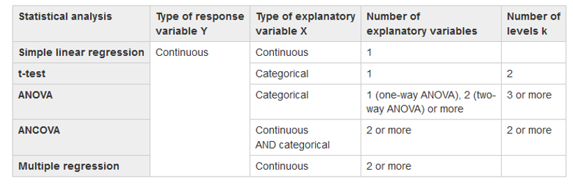
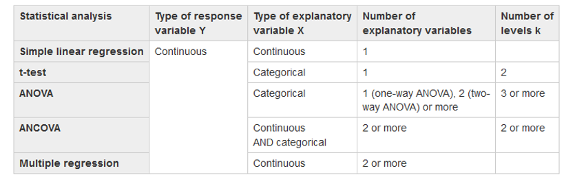
Create plots of your data picking 2 variables that are continuous, then create a linear model (regression) using your data. Use this Table as a guide Create a simple linear model using lm() lmb <- lm(y ~ x, data = mydata) |
 |
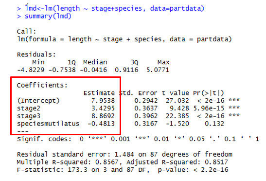
lm() = Linear Model Function lmb <- lm(length ~ width, data = mydata) Use these functions to interogate your model! summary(lmb) Estimates goodness of fit, significance anova(lmb) familiar anova table str(lmb) structure of lmb object, or what is in the object |
Here is the General Output 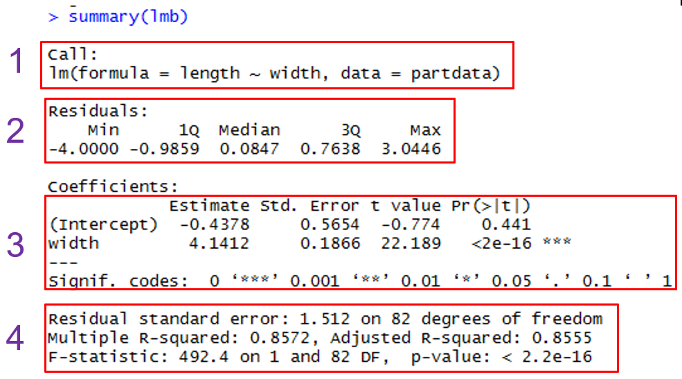 |
13.5 Diagnostics
These are applicable to just about all GLMs.
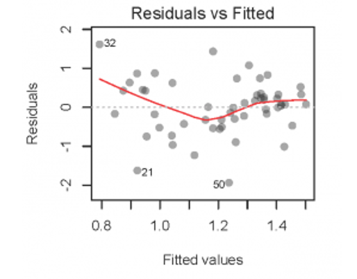
Mainly plots to look at residuals.
- Residuals vs. Fitted Values (verify homogeneity)
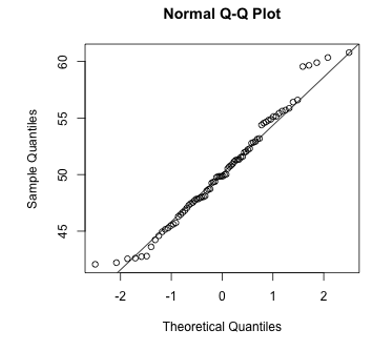
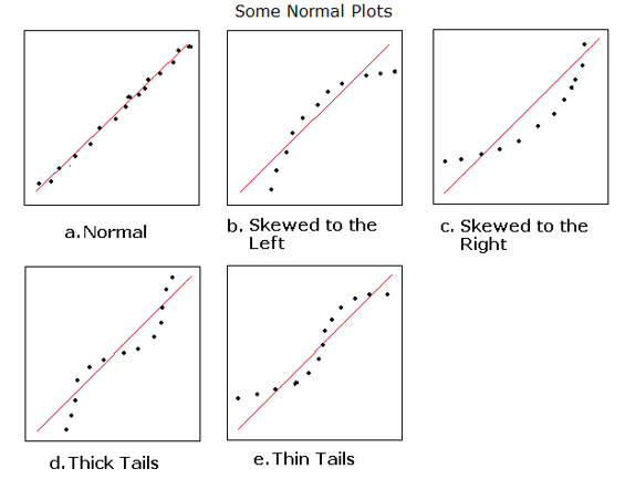
- Q-Q Plot of Histogram of Residuals (normality of errors)
- Residuals vs. Explanatory (x) (Independence)
- Influential Observations
We will use the simple plot functions
13.5.0.1 Homogeneity
Tests can be used for this, but Beware!!!
# Bartlett Test of Homogeneity of Variances
bartlett.test(length ~ stage, data = mydata)

# Figner-Killeen Test of Homogeneity of Variances
fligner.test(length ~ stage, data = mydata)
It is better to plot the fitted vs. residual values!
plot(lmb) will produce 4 plots, but we can do this manually too!

13.6 Plot Your Model
Let’s look at some examples of plotting your data using the ggeffects package!
#Plot the relationship
ggplot(mydata, aes(x = x_variable, y = y_variable))+
  geom_point()

# linear model
M1<-lm(y ~ x, data = mydata, na.action = na.exclude)

predict_response(M1)%>%plot(show_data=TRUE, ci_style = "errorbar", dot_size = 1.5)
predict_response(M1)%>%plot(ci_style = "errorbar", dot_size = 1.5)

#Add residuals
#This method works on simple models and appends residuals to mydata
mydata<-mydata%>%
  add_residuals(M1)%>%
  add_predictions(M1)

#Plot residuals
#There is a lot more to do here...this is an example
ggplot(mydata)+
  geom_histogram(aes(x=resid), fill='grey50', col='black')+
  theme_bw(22)+ylab("Frequency")+xlab("Residuals")

ggplot(mydata)+
  geom_boxplot(aes(x=common_name,y=resid), fill='grey50', col='black')+
  theme_bw(22)+ylab("Residuals")+xlab("Common Name")

ggplot(mydata)+
  geom_point(aes(x=pred,y=resid), fill='grey50', col='black')+
  theme_bw(22)+ylab("Residuals")+xlab("Predicted")
13.7 Model Specification in R
When modelling in R, glm specification can look like this:
Here’s what these mean:
- y = response variable
- x1 = first explanatory/predictor variable
- x2 = second explanatory variable
- x3 = third explanatory variable
*= include ALL interaction effects (for the two joined)+= include only main effects (no interactions):= specific interaction effects
Note: x1/x2 is read as x2 nested within x1
13.8 Extending Models
Models are extended by adding more explanatory variables.
Explanatory variables are called covariates.
Recall an example:
If x2 is a continuous variable, the model is a multiple regression.
If x2 is a categorical variable, the model has both a regression variable (x1) and a categorical variable (x2).
Let’s look at some classical model specifications!
13.8.0.1 Multiple Regression
Here width and weight are both continuous.
Finds the relationship between length and both width and weight!
# Multiple Linear Regression Example
lmc <- lm(length ~ width + weight, data = mydata)
summary(lmc) # show results

# Other useful functions
coefficients() # model coefficients
confint(lmc, level = 0.95) # CIs for model parameters
anova() # anova table
vcov() # covariance matrix for model parameters
influence() # regression diagnostics
13.8.0.2 ANOVA
What if the covariate is a category?
Q: Are species lengths different?
# One Way Anova (Completely Randomized Design)
predict <- aov(y ~ A, data = mydata) # A is a factor

# Two Way Factorial Design
predict <- aov(y ~ A + B + A:B, data = mydata) #A and B are factors
predict <- aov(y ~ A * B, data = mydata) # same thing
Notes:
aov() is the ANOVA wrapper for lm() and it has to be balanced
glm() is more general and unbalanced designs are acceptable
Balanced is where each category has the same number of observations
Create an ANOVA using your data picking 1 variable that is continuous and 1 variable that is categorical
Use this table as a guide:
Create a simple linear model using aov()
13.9 GLM
Creat a GLM using your data picking 1 variable that is continuous and 1 variable that is categorical
Create a simple model using glm()
Try your ANOVA!
Create a more complex model using glm()
Run diagnostics (plots etc) on your models.
13.10 Comparing Models
Great! So we can specify many different models mixing covariates of different types (e.g. categorical and continuous; there are other types too!)
How are models compared?
anova(model1, model2, model3, …, test = “F”) #likelihood ratio
drop1(model1) # drops each term in order
AIC(model1, model2, model3, …)
BIC(model1, model2, model3, …)
lrtest(model1, model2)
vuong(model1, model2)
Parsimonious models are preferable to big models if both have similar predictive power.
A parsimonious model is one with the fewest predictors and significantly better than models with more predictors.
If models are not nested, sometimes cannot use the F-test to choose between one and another. Must rely on other sample statistics such as \(R^{2}\) and RMSE. Or can use the Vuong test.
In the end, choice of any model is subjective…
13.11 Hypothesis Testing
Let’s go through an example using the ggeffects package!
#Continuous and Categorical Interaction Effects Regression Model
#Main effects only
#This means a common slope estimate across common_name
M2<-lm(continuous_variable~categorical_var1+categorical_var2, data = mydata)

# You can also try this in the model too!
#Include interaction effects (use * in place of +)
#This means a separate slope estimate for each common_name

# let's plot it!
ggpredict(M2, terms = c("categorical_var1", "categorical_var2"))%>%plot()

# Now let's test the hypothesis!!
test_predictions(M4, terms = c("categorical_var1", "categorical_var2"), test=NULL, p_adjust = "tukey")
test_predictions(M4, terms = c("categorical_var1", "categorical_var2"), p_adjust = "tukey")