Chapter 12 Intro to Modelling
12.1 Review of Linear Regression
12.1.0.1 Linear Relationships
Our goal here is to display relationships between variables, or to describe the linear relationship between x and y and to predict x from y. Equation of a straight line: \(y = \beta_{o} + \beta_{1}x\) \(\beta_{o} = y_{intercept}\) \(\beta_{1} = slope\) \(slope = \frac{rise}{run}\) |
 |
12.1.0.3 Regression Lines
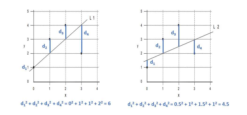
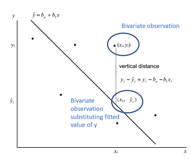
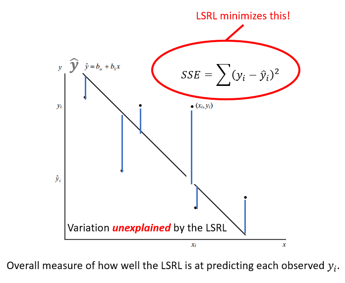
Given a bivariate sample \((x_{i},y_{i}) ... (x_{n},y_{n})\) The vertical drop is given by: \(y_{i} - \hat{y}_{i} = y_{i} - b_{0} - b_{1}x_{i}\) \(\hat{y}_{i} = b_{0} - b_{1}x_{i}\) are the fitted values (and form the line) The least squares line is the line that minimizes: \(\sum(y_{i} - b_{0} - b_{1}x_{i})^{2}\) or more simply \(\sum(y_{i} - \hat{y}_{i})^{2}\) Over all possible choices of \(b_{0}\) and \(b_{1}\) That is, if we randomly chose many \(b_{0}\) and many \(b_{1}\), say 100,000 we may happen upon the exact values However, both \(b_{0}\) and \(b_{1}\) can be calculated! |
 |
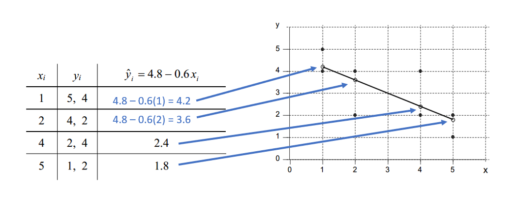
| For any \(x_{i}\) there may be more than one \(y_{i}\), but each \(\hat{y}_{i}\) receives the same estimate! Here’s an example! |
 |
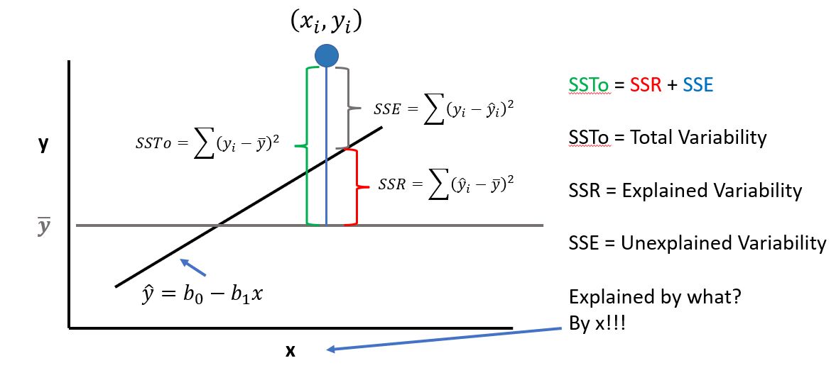
12.1.0.4 Assessing the Fit of a LSRL
The LSRL is a good fit if the sample points \((x_{i},y_{i})\) along the LSRL defined by \(\hat{y} = b_{0} - B{1}x\) is much better than \(\overline{y}\) (mean value of all \(y_{i}\)) at predicting the observed \(y_{i}\) Or (equivalently) if the total variation in the \(y_{i}\) values is well exxplained by the LSRL! Recall: A residual is also called an error with symbol e. \[e = (y_{i} - \hat{y}_{i})\] Summing all squared errors gives the variation unexplained by the LSRL. We call this error variation the Error of Sum of Squares (SSE) |
 |
12.2 Models Introduction
12.2.0.1 General Considerations
In general, our hypotheses are about relationships between concepts or things.
Concepts can be measured, so we can test relationships between variables
- Concepts can be a target organism, environmental state, etc.
- Variables represent what is being measured
Modeling is:
- Describing the relationship between variables
- Describing how the things are measured aka how the data is generated
A model takes both into account
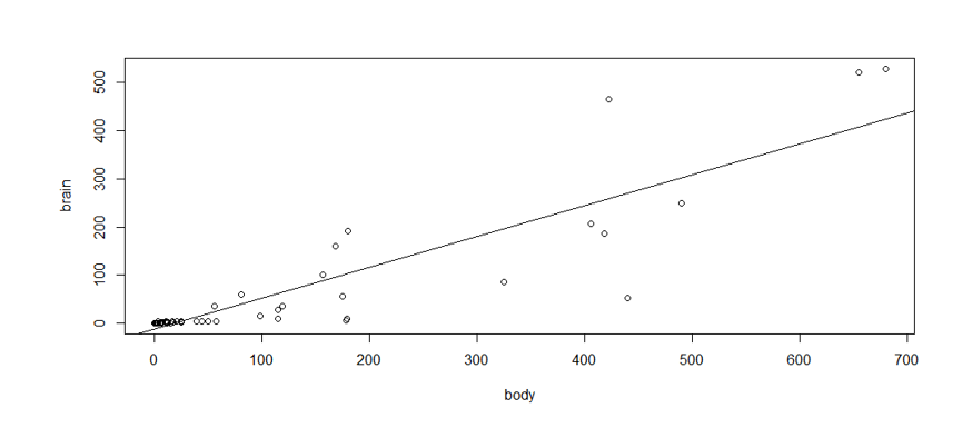
Suppose we want to describe the relationship between mammal body size (in weight) and brain weight
Hypothesis: Larger mammals have larger brains
- We measure body weight and brain weight
- We create a simple linear model; in this case a linear regression
- There is variability about the relationship
Like this:
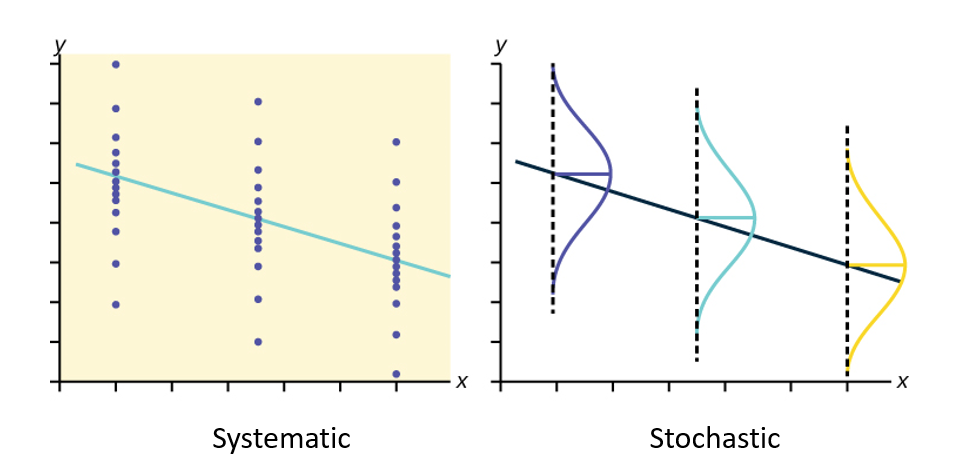
The model, then, the total variation of brain weight consists of:
- A systematic component: how brain wt varies as a function of body wt
- A Stochaistic component: variability due to other causes, which we can not explain with our data
A model is a summary of the data in terms of the systematic effect + a summary of the magnitude of the unexplained or random variation!
12.2.0.2 Model Components
Systematic component
- Defines the relationship between X and Y (between body wt and brain wt)
- It represents the variation of body wt to explain the variation of brain wt
- This idea (relationship of X and Y) is what our hypotheses are (usually) about
Stochastic component
- Defines the distribution of Y
- It describes the variation of brain wt
- In the absence of predictors (variables that we think might explain Y), all variation in brain wt is stochastic
- We specify this component by making assumptions about the statistical process that generated the values of brain wt (**In linear models it is assumed to be normal*)
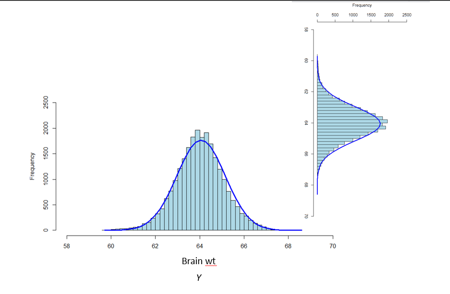
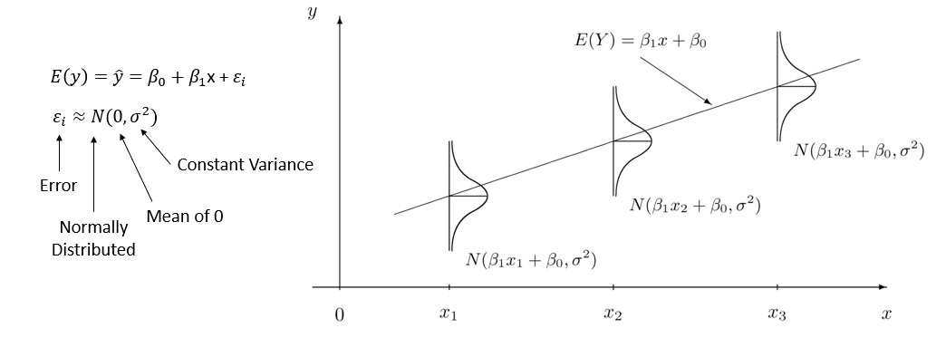
Here is a visual of the different model components we just discussed:
Put it all together:
Quick Summary:
- A linear model is an assumption about the nature of the relationship between body wt and brain wt
- It describes how much brain wt changes on average for a unit increase in body wt
- It also describes how much of the variation in brain wt is not explained by body wt
12.2.0.3 Modeling Probabilities with GLM
How can we work a binary or probability response with GLM?
- We need to transform the probability of Y (i.e. the mean of Y) in a way such that it can be related to X linearly
- This is done using a mathematical function called link function
- The link function transforms a probability into a quantity called linear predictor
- The linear predictor is the systematic component of the model, and can be modeled in the same way as in simple linear models like simple linear regression
12.2.0.4 GLMs in Brief
- Specify the distribution of the dependent variable
- This is the assumption about how the data are generated
- This is the stochastic component of the model
- Specify the link function
- We linearize the mean of Y by transforming it into the linear predictor
- It always has an inverse function called response function
- Specify how the linear predictor relates to the independent variables
- This is done in the same way as with linear regression
- This is the systematic component of the model
12.3 GLMs in Practice
12.3.0.1 Residuals
In textbooks and online, you will note different words being used for the same items within modeling.
Here is a guideline:
- Ordinary (raw) residuals = response residuals
- Observed value - fitted value
- Pearson residuals
- Standardized ordinary residuals
- Ordinary residuals/sqrt(fitted mean) there are others
- Deviance residuals (default in R)
- Quantify the contribution of each observation to the residual deviance
- Use for zero-inflated and binomial distributions
- When in doubt, use deviance residuals!
- Studentized residuals
- Normalized residuals
12.3.0.2 Summary of GLM Process
Once you create your model, you aren’t done (Sadly)! We need to go over and interprete the model, validate it, and make sure the relationships between our variables are being described appropriately and accurately.
Let’s go over the process!
12.3.0.3 1. Fitting
When you first fit your model, you need to do an initial interpretation. Then you move into validating your model!
Let’s go over the steps for Validating a GLM
- Homogeneity of error variance
- Independence
- Inherent dependency (E.g. repeated observations on units)
- Dependency due to model misfit (Missing a covariate)
- Normality of Residuals (not your data!!!!)
- Influential observations
- Plot residuals vs.
- Covariates included and excluded
- Time and/or space
- Fitted values
- Dispersion (overdispersion or underdispersion) Only for count models
- Biological sense??
12.3.0.4 2. Visualization
- Plot your model
- Interpret the plot
- Does it make biological sense now?? (No? Repeat)
12.3.0.5 3. Interpretation
After you go through those steps (Again, you may need to repeat the validation process a few times), you then need to finalize the model and your interpretation of it in relation to your variables!
Remember: All data is different, some models might not be the best fit for your data
We can always go back to step 1 and try a new fit, and then walk through the validation steps again. There is no limit.
12.4 GLM Demo
Let’s do an example and walk through it together!
This example is taken from Zuur et al. 2013 Beginner’s Guide to GLM and GLMM in R.
- The data are fisheries data from two periods – pre-commercial, and post-commercial fishing.
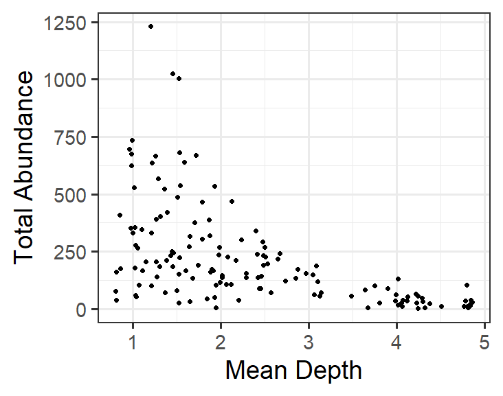
- Response variable = Total Abundance of all species
- Explanatory variable #1 = Depth (m) (range 800-4000+ m)
- Explanatory variable #2 = Period (categorical, 2 levels)
12.4.0.1 Step 1 - Fit the Model
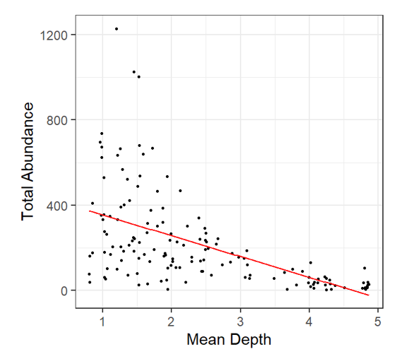
Visualizing the relationship between Total Abundance and Depth is straightforward. Always start simply when modeling!
Here is what is would look like in R:
This model corresponds to:
\[TotAbund = β_{1} + β_{2} * MeanDepth_{i} + \epsilon_{i}\] where the model estimates \(TotAbund\) at \(MeanDepth_{i}\)
remember that \(_{i}\) is each point in the data.
12.4.0.2 Step 2 - Validate Model
Several validation steps are done for each model. Here is the list again, in a logical order.
- Check for normality of residuals.
- Check for homogeneity (homoscedasticity) of residuals.
- Check for independence of each value.
- Check for influential observations.
- Check if the model makes biological sense.
Assessing a model for biological sense is quite important.
If the model does not predict values of the response (realized values) that are biologically meaningful, then the model does not fit the data and a different model should be used.
To validate the model residuals:
- Extract the residuals from the model object. In this case we will use ordinary residuals, but deviance would work well too.
- Plot residual diagnostic plots.
- Assess whether the residual relationship to fitted values is realistic.
- Also plot residual relationship to all covariates within the model or not in the model. (More on this later).
- Assess realized values. One way to do this is to simulate Total Abundance at various (and user-selected) points of Depth
- This is somewhat complicated, but is used to demonstrate a couple of vary important points!
Let’s see how this would look!
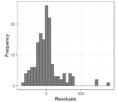
| Check for the Normality of Residuals | |
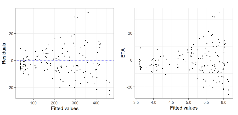
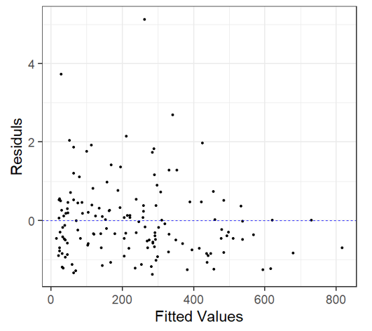
E0 <- resid(M0) # Residuals F0 <- fitted(M0) # Fitted Values Let’s look at the residual plot |
 |
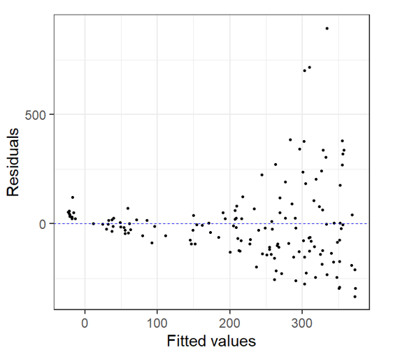
Residual v. Fitted Heterogeneity in the residuals: i.e. higher variation in the residuals for larger fitted values Non-linear patterns in residuals: groups of residuals clustered at less than zero and also greater than zero. |
 |
| Does it Make Biological Sense?? | |
In this case, after we look at the residual plots we can go back and take another look by plotting the Total Abundance vs. Mean Depth with model fit line: Here’s is what we notice: At depths close to 5 km, fitted data becomes negative This does not make biological sense! |
 |
Let’s plot the Model fit with simulated total abundance values Black dots: observed data Grey dots: simulated data Again, negative total abundance values do not make biological sense! |
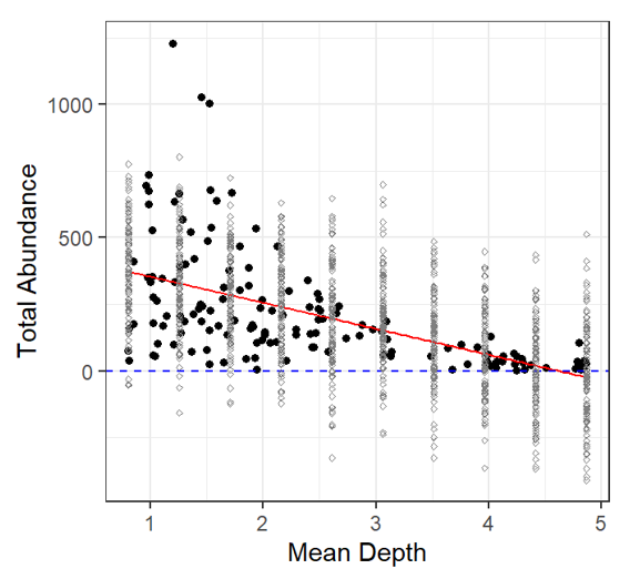 |
12.4.0.3 Validation Summary
To sum up:
- Residuals appear to be more/less normally distributed.
- Does this mean the errors are normally distributed?
- Residuals were heteroscedastic (heterogeneous) and showed patterns
- Even though the residuals are normally distributed about Depth points, they also predict negative Total Abundance values (negative realizations)
- The model also predicts negative Total Abundance fitted values which is biologically ridiculous.
So, this model is CRAP!
What is the issue?
The response variable is count data. Count data do not follow a Normal (Guassian) distribution, instead, count data follow a Poisson distribution! Let’s try to model it!
To do this, we require:
- A distribution for the response variable.
- A predictor function specifying the covariates.
- The link between the predictor function and the mean of the distribution. (we mentioned these earlier!)
In our example, TotAbund is the response variable. It:
- Likely follows a Poisson distribution,
- Is related to the covariate MeanDepth, but also could be related to other covariates (i.e. other variables), and
- Likely requires a link function to prevent realized values that are negative.
12.4.0.4 Link Functions
It makes sense to use a probability distribution that fits with the data type being modeled.
The data are count data and count data often follow either a Poisson or Negative Binomial distribution. Why?
Poisson distributions have a simple property in that the mean is equal to the variance.
So, we have determined that the responses probably follow a Poisson distribution. Set that aside.
What about this ‘link’ function?
When we used the linear model, the mean TotAbund response is what is being fitted at each point of Depth using a defined predictor function \(\beta_{1} + \beta_{2} * MeanDepth_{i}\) which we can write as:
\[\eta_{i} = \beta_{1} + \beta_{2} * MeanDepth_{i}\]
Where \(\eta_{i}\) is our predictor function.
What we want to do is link \(\mu_{i}\) (the mean) to the predictor function \(\eta_{i}\) in a useful way.
Identity link
\(\mu_{i} = \eta_{i}\)
So, the mean response along the regression line is the estimate
\(\hat{y_{i}}\) along the line (the mean at \(x_{i}\)).
Log link
The advantage of the log link is that values will always be positive. This is precisely what we want with this model!
\(\log(\mu_{i}) = \eta_{i}\)
${i} = e^{{i}} = e^{{1} + {2} * MeanDepth_{i}} $
GLM Families
Specifying a different modeling distribution is rather easy.
| Family | Default Link Function |
|---|---|
binomial |
(link = "logit") |
gaussian |
(link = "identity) |
Gamma |
(link - "inverse") |
inverse.gaussian |
(link = "1/mu^2") |
poisson |
(link = "log") |
quasi |
(link = "identity", variance = "constant") |
quasibinomial |
(link = "logit") |
quasipoisson |
(link = "log") |
12.4.0.5 Poisson Distribution
\[\mathrm{P}(X = k) = \frac{\lambda^{k} 𝒆^{−\lambda}}{k!}\] \[\lambda = \mathrm{E}(X) = V(X)\] Let’s see how our model specification fits into these formulas!
\[TotAbun_{i} = \beta_{1} + \beta_{2} * MeanDepth_{i} + \varepsilon_{i}\]
\[\varepsilon_{i} \sim N(0, \sigma^{2})\]
Same Gaussian model, different specification:
\[TotAbun_{i} \sim N(\mu_{i}, \sigma^2)\] \[E(TotAbun_{i}) = \mu_{i}\] \[var(TotAbun_{i}) = \sigma^{2}\] \[\mu_{i} = \beta_{1} + \beta_{2} * MeanDpeth_{i}\]
Poisson model
\[TotAbun_{i} \sim P(\mu_{i})\] \[E(TotAbun_{i}) = var(TotAbun_{i}) = \mu_{i}\] \[\eta_{i} = \beta_{1} + \beta_{2} * MeanDepth_{i}\]
Using a link between the mean value of \(\mu_{i}\) and the covariates
\[\mu_{i} = \eta_{i}\]
But, the link function can still produce negative values, so:
\[\log(\mu_{i}) = \eta_{i}\] \[\mu_{i} = e^{n_{i}} = e^{\beta_{1} + \beta_{2} * MeanDepth_{i}}\]
12.4.0.6 Step 3 - Try it Again
We have now established:
- A Poisson distribution is probably useful
- A log link corresponds to our model (positive responses only).
So, let’s try a new model:
Note: The default link for family poisson is the log link (so we don’t need to specify it).
And now Let’s begin again with model validation (residuals, plots, etc.)
Once the validation process indicates no issues, we follow it with model interpretation.
Residual v. Fitted Heterogeneity in the residuals: Again, we see that the residual plots are not ideal! |
 |
The fitted line plot with simulated values added (just like in the linear model), shows no negative predictions, yay Black dots: observed data Grey dots: simulated data Red line: fitted values of Poisson GLM Makes biological sense! BUT |
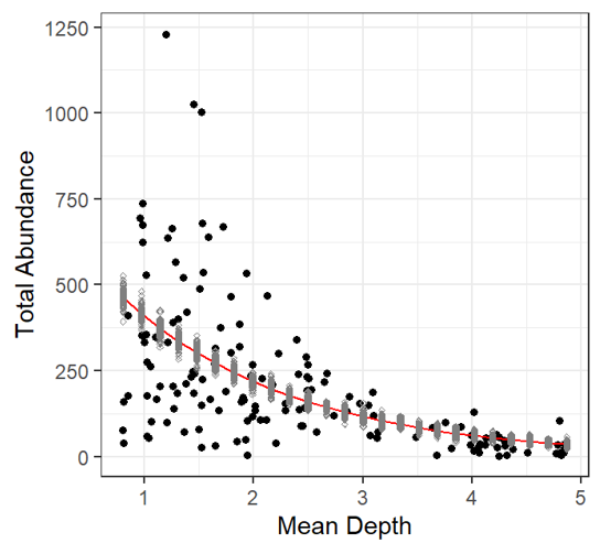 |
12.4.0.7 Validation 2 Summary
There is another issue:
The data (observations) are more dispersed than the model predicts!
This result is known as overdispersion, and it is a very important thing to investigate. It occurs with Poisson family distributions.
Luckily, we have created some functions to help with calculating dispersion.
To sum up:
- Residuals were heterogeneous and showed patterns,
- Residuals are normally distributed about Depth points, but they are more dispersed than the Poisson model predicts.
So, this model is CRAP! (again)
12.4.0.8 Dispersion
Overdispersion can be caused by:
- Missing explanatory variable(s)
- One or more outliers
- Missing interaction term(s)
- One (or more) explanatory variables on the wrong scale (need to be logged, squared, etc.)
- Non-linear effects of a continuous covariate
- Mis-specified model (incorrect link function)
- Zero-inflation
- Inherent dependency structure in the data
Investigating each of these may reduce dispersion, but what level is correct?
Very fine statisticians have simulated Poisson model outcomes, and have determined that a dispersion of 1 realizes a perfectly fitted Poisson model.
- Dispersion statistic >1: overdispersed
- Dispersion statistic <1: underdispersed
Therefore, let’s try to get to a dispersion of 1.
- Look for outliers
- Add a covariate (Period), and look at others (spatial covariate)
- Try a different distribution - The Negative Binomial
Let’s Investigate
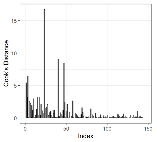
| Cooks Distance | |
Cooks distance may be used to determine outliers! Cook’s distance values >1 may be influential to the model. But there are over 20 values >1! We cannot exclude all of these observations. Dispersion is still high when we remove largest outlier |
 |
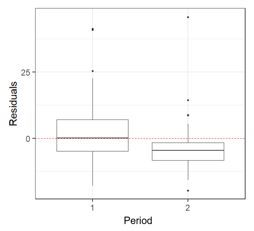
| Adding a Factor | |
This plot indicates that there is a Period effect on the residuals. So we should add period as a factor in our model To determine if the depth effect on abundance changes per period, we need to add an interaction between Mean Depth and Period dispersion(M2) 111.1873 **There is still overdispersion in this model, what now? |
 |
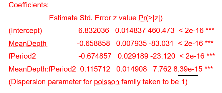
Adjust for sample period! dispersion(M2) 111.1873 The interaction factor is significant, but there is still too much overdispersion… |
 |
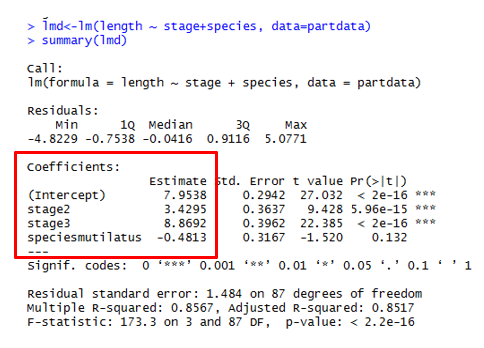
| Coefficients | |
Coefficients MUST BE CALCULATED! Intercept <- Intercept (first value of each factor) i.e. \(stage1 = 7.95\) \(speciesmicans = 7.95\) \(stage2 = 7.95 + 3.43 = 11.38\) \(stage3 = 7.95 + 8.87 = 16.82\) \(speciesmutilatus = 7.95 - 0.48\) \(stage2 = 7.95 - 0.48 + 3.43\) \(stage3 = 7.95 - 0.48 + 8.87\) |
 |
12.4.0.9 Negative Binomial
Negative binomial distribution contains a second parameter called the dispersion parameter or heterogeneity parameter used to accommodate Poisson overdispersion.
The previous modelling results indicated that variance is larger than the mean, so a negative binomial distribution may fix this overdispersion.
Model Specification |
\(TotAbun_{i} = \beta_{1} + \beta_{2} * MeanDepth + \varepsilon_{i}\) \(\varepsilon_{i} \sim N(0, \sigma^{2})\) |
| Poisson Model | \(TotAbun_{i} \sim P(\mu_{i})\) \(E(TotAbun_{i}) = var(TotAbun_{i}) = \mu_{i}\) \(\eta_{i} = \beta_{1} + \beta_{2} * MeanDepth_{i}\) |
| Using a link between the mean value of \(\mu_{i}\) and the covariates \(\mu_{i} = \eta_{i}\) But, the link function can still produce negative values, so: \(\log(\mu_{i}) = \eta_{i}\) or \(\mu_{i} = e^{\eta_{i}} = e^{\beta_{1} + \beta_{2} * MeanDepth_{i}}\) |
|
Negative binomial Model Note: It includes the additional factor, Period as well |
\(TotAbun_{i} \sim NB(\mu_{i}, k)\) \(E(TotAbun_{i}) = \mu_{i}\) and \(var(TotAbun_{i}) = \mu_{i} + \frac{\mu_{i}^{2}}{k} = \mu_{i} + \sigma + \mu_{i}^{2}\) \(\log(\mu_{i}) = \eta_{i}\) \(\eta_{i} = \beta_{1} + \beta_{2}xMeanDepth_{i} + \beta_{3}xPeriod_{j} +\beta_{4}xMeanDepth_{i}xPeriod_{j}\) |
Negative Binomial Distribution dispersion(M4, modeltype = 'nb’) [1] 1.001618 The dispersion statistic is essentially 1! |
 |